Experts debate endlessly about the direct use of M language, which is the script language behind Power Query.
The Power Query tool is a UI in front of the M language. This UI is covering more and more areas of functionality, but there is still a lot more power locked in the language. This leads to some people turning to straight use of the M language. A great example from way back when Power Query was not even called Power Query is this article from Chris Web (2013).
Many times in the past, I told people, “Instead of learning M, get a life.” What I meant was that M is hard, and Power Query is already very rich; therefore, spend your time learning more useful tools such as DAX.
Nowadays, I’m more open to a limited kind of using M that tweaks the generated M, as opposed to actually writing new M statements.
Anytime you find yourself opening the Advanced Editor, ask yourself if you have a good reason for that, and if the person that will need to maintain this solution after you will be able to follow what you did. If you apply some tweaking on the formula bar, you are probably in a safe place.
That is why I was happy to see that I can a solve a non-trivial problem without opening the Advanced Editor once.
Task on hand
I created a dataset with annual total sales for customers. The original dataset was much larger and came from a slow web source.
Every customer/year combination has a row, but many rows have zero as the value. I want to filter all the rows that have zero as the value, but after the filter, my pivoted results are skewed.
I pivot on year, and if the first customer has non-empty data for 2005 and 2008 and the second customer for 2006 and 2009, the order of columns of the result pivot will be 2005, 2008, 2006 and 2009. If no customers have data for a specific year, this year will be absent from the pivoted result. In this dataset, there are no sales for 2009.
I want all years to appear in the pivot and in the right order. On the other hand, I want to filter out the rows with zero values in order to read less rows from the source.
The solution I came up with leaves all data for the first customer and removes empty rows from all other customers. In this way, all years are represented for the first customer and appear in the right order in the pivot. (Input data is sorted by customer and year.)
Steps
First, I want to extract the key of the first customer. The data is already in the Excel file, so I start a query from table. Instead of continuing with the rest of steps, I remove all but the first row, right-click the customer field and then right-click/drill down. This creates a simple value named Customer with a value of C1, which is the first customer key.
Now I need to continue with the regular steps, so I insert a new step from the Fx icon in the formula bar. I change the created line to = Source, which brings back the table with all rows in the original Excel table.
Now I filter on two columns: Amount <> 0 and Customer= “C1”
The generated line I see in the formula bar is:
= Table.SelectRows(Custom1, each ([Amount] <> 0) and ([Customer] = “C1”))
The tweak : I change the “and” to “or” and the second filter argument to use Customer, which is the variable I created in the beginning:
= Table.SelectRows(Custom1, each ([Amount] <> 0) or ([Customer] = Customer))
This filter cannot be created from the UI because it combines filtering on two different columns with an “or” condition and also uses a variable for comparison. It is still pretty easy to read and understand.
I want all rows from the first customer and all other non-zero rows. This guarantees that all years are found and in the right order, as you can see in the pivoted result.
So the two kinds of tweaks are the second use of source in the query and the manual change to the filter expression. The UI was nice enough to combine filtering on two columns to one filter statement and I changed the “and” between two columns to “or” and the filter operand from a fixed value to a variable one.
In my opinion, this level of tweaking is acceptable, and balances the need to create clear and maintainable solutions and the geeky urge to use more of the power of the M engine.
Power Query FAQ
Power Query is a function of Microsoft Excel that allows users to import data from various sources and sorts them into an excel sheet in the most convenient and usable way. Users only need to program instructions into Power Query a single time and then the query will repeat the same commands when prompted every time thereafter.
The unique aspect of Power Query is that it does not require a working knowledge of coding to execute. Users only need to be comfortable in Excel and know the Power Query functionality. It is a Business Intelligence tool that can increase productivity.
Power Query has the ability to execute various functions that end-users historically had to do on their own. Data is pulled from sources into one spreadsheet which Power Query can then filter, sort, and edit based on user-programmed input.
Some of the more beneficial functions are:
● Split Cells Using A Delimiter – typically cells with data separated by commas, semicolons, or dashes.
Correct Formatting Specific To Country – usually used to correct foreign representations of currency.
Complete Missing Data – used when data is exported from a source that does not have all columns completed.
● Group Data – allows for the summarization of multiple data sets.
(images from goskills.com)
Power Query allows users to filter rows based on a value that is inside a column. There are many ways to filter rows in Power Query, below are some examples.
Filter Using AutoFilter Function
Autofilter is a function in Power Query that finds, hides, or shows values and allows users to specify filter criteria more easily. To use AutoFilter follow these steps:
Open a query, select a cell in the dataset, and select Query > Edit.
Select the icon next to the column that you would like to filter
Select each checkbox next to the corresponding value you would like to filter and select OK.
Filter By Row Position
Users can filter rows by position, which will either include or exclude rows based on their position in the dataset.
To Keep Top Rows
Open a query from the Power Query Editor, select any cell in the data and click Query > Edit.
Click Home > Keep Rows > Keep Top Rows
A dialogue box will open, enter the number of rows you wish to keep starting from the top and moving down.
Click OK.
To Keep Bottom Rows
Open a query from the Power Query Editor, select any cell in the data and click Query > Edit.
Click Home > Keep Rows > Keep Bottom Rows
A dialogue box will open, enter the number of rows you wish to keep starting from the bottom and moving up.
Click OK.
To Keep A Range Of Rows
Open a query from the Power Query Editor, select any cell in the data and click Data > Query > Edit.
Click Home > Keep Rows > Keep Range of Rows
A dialogue box will open, enter the value for the first row and the number of rows you wish to keep. For example, if your dataset begins on row 9, then put nine for First Row and then the number of rows you wish to keep.
Click OK
Pivot And Aggregate A Column
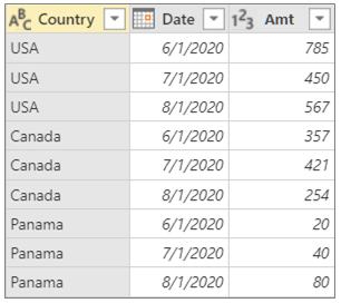
Using the Dataset below we will pivot the data and aggregate the results into a new column.
1. Open a query from the Power Query Editor, select any cell in the data and click Query > Edit.
2. Choose the column that you would like to pivot against. In this example, we will use “Date”, which will become the values of the new columns and headers.
3. Click Transform and then Pivot Column
4. A dialogue box will open, in the Values column list, select which column value you would like to pivot. For this example, we will select Amt, which is the third column in the example data set.
5. Click Advanced Options and click the function button that says Aggregate Value. You will be prompted with several options to choose from. For this example, choose the sum option.
6. Click OK.
Resulting pivot:
(Images from microsoft.com)
In Excel, open Power Query Editor by clicking Launch Query Editor found by navigating to Data > Get Data > Launch Power Query Editor. The functionality allows users to import or, in some cases, connect to external data sources. This allows users to reshape data that is being fed directly to excel.
Certain circumstances require users to combine multiple tables into one concise dataset. Power Query can be used to merge various tables into one unified table without the use of VLOOKUP.
To do this follow these steps:
1. Select any cell in the table that you would like to merge
2. Navigate to Data > Get Data
3. Here you can select Other Sources > From Table/Range
4. Select the table range of your source data, this will pull the table into the open Excel file in a new table that will update as the source table does
5. To merge tables navigate to Data > Get Data > Combine Queries > Merge
6. Select the tables you would like that have a matching column. Select the Join Kind and click OK
Some models pull in a great deal of data and as a result, the refresh times can become exaggerated. In order to reduce lag times and increase the speed at which Power Query refreshes consider what part is slow. Slowdowns are typically caused by data refreshing, model calculations, visualizations, and graphics, but there are other causes as well.
One common issue is problems with query folding, so be sure to verify that your query folding is working correctly. Folding is the process of taking tasks generated by the Power Query user interface and sending those tasks to a database for execution. Confirm this is working properly by right-clicking on any step and selecting View Native Query and check for any broken steps that break the query process.
Also, consider minimizing the amount of data that the query pulls by eliminating unused columns or rows. The same can be done with formulas, minimizing calculations where possible to free up resource demand.
1. Open Excel and select and navigate to File > Options
2. Choose Add-Ins > Manage drop-down menu > COM Add-Ins > Go
3. Next look for the Power Query option in the available add-ins. Select the box next to it and click OK.
4. Reboot Excel
Datarails replaces spreadsheets with real-time data and integrates fragmented workbooks and data sources into one centralized location. This allows users to work in the comfort of Microsoft Excel with the support of a much more sophisticated data management system at their disposal.
Every finance department knows how tedious building a budget and forecast can be. Integrating cash flow forecasts with real-time data and up-to-date budgets is a powerful tool that makes forecasting cash easier, more efficient, and shifts the focus to cash analytics.
Regardless of the budgeting approach your organization adopts, it requires big data to ensure accuracy, timely execution, and of course, monitoring.
Datarails is an enhanced data management tool that can help your team create and monitor cash flow against budgets faster and more accurately than ever before.
Learn more about the benefits of Datarails here.


