
Key Takeaways: Data Consolidation in Excel
- Excel’s Consolidation Capabilities: Excel includes built-in tools, such as the Consolidate function, that let finance teams summarize data from multiple sheets or files. It remains popular for its flexibility and ease of use.
- How to Consolidate Data in Excel (Common Methods): Data can be combined using the Consolidate tool, formulas (including 3-D references), PivotTables, or Power Query. The best method depends on your data structure and complexity.
- When Excel Works Best: Excel is well-suited for small to mid-sized datasets, limited sources, and consistent formats. It’s effective for monthly or one-time consolidations without heavy automation needs.
- Challenges of Excel Consolidation: Manual consolidation in Excel can lead to broken links, version issues, and errors. It struggles with large datasets and doesn’t support real-time collaboration or audit trails.
- Modern Solutions Beyond Excel: Finance teams now pair Excel with FP&A platforms like Datarails that pull data from multiple systems and feed it into reports automatically. This improves accuracy and reduces manual work.
Excel remains one of the most widely used tools for financial analysis, and for good reason. It’s flexible, familiar, and powerful enough to handle many consolidation tasks.
However, as data volumes grow and sources multiply, manually consolidating data in Excel can become a fraught and time-consuming process.
Finance teams often spend hours copying and pasting data across multiple sheets or files, reconciling formatting mismatches, fixing broken formulas, and revalidating numbers after every update.
The problem isn’t Excel itself; it’s how far teams try to stretch it.
Knowing how to consolidate data in Excel properly (and recognizing when Excel starts to break down) is critical to maintaining accuracy, speed, and confidence in financial reporting.
This guide covers the most common Excel consolidation methods, when to use each one, and how modern finance teams reduce risk by combining Excel with more sophisticated, automated data consolidation solutions.
What is Data Consolidation in Excel?
Data Consolidation is an Excel feature that enables you to collect data from different worksheets and compile it in one, centralized sheet.
I It creates a ‘master’ table where you can access data summarized from other sheets. The result? Your information becomes much easier to read and understand in its new aggregated form.
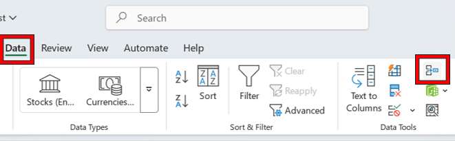
Excel makes this possible through the ‘Consolidate’ tool, located under the “Data” tab.
A handy function for FP&A analysts, it has been around for over two decades. Its main function is simple: combining information from several worksheets or workbooks and displaying it in a neat summary. Located under the “Data” tab
But it works only if the data you want to consolidate has a single column and a single row of labels and headings, respectively.
While this can seem like a major drawback, most datasets you’ll encounter will follow this format.
Financial analysts use consolidation for tasks such as:
- Combining actuals, budgets, and forecasts from different departments
- Aggregating monthly sales or expense reports into a summary
- Rolling up multi-entity financials into a consolidated statement
Essentially, whenever you have similar data split across multiple sources and need an overall summary, that’s a scenario for data consolidation.
For instance, combining budgets from various departments into one company-wide budget is a classic example of using Excel’s consolidate function.
Of course, it’s important to distinguish between consolidation and aggregation.
In Excel terms, “consolidation” often implies bringing data together (possibly from multiple sheets/files) and summarizing it.
Aggregation is the mathematical summarization itself (summing up numbers, taking averages, etc.).
In practice, the Excel Consolidate feature performs aggregation of data across different sources.
A related concept is using a PivotTable to aggregate data by categories. Pivoting is a more flexible way to consolidate by categories (labels) if your analysis needs to be interactive or more detailed.
When Excel Is a Good Tool for Data Consolidation
Excel shines as a consolidation tool in certain scenarios. Knowing when Excel is suitable for data consolidation can save time and prevent frustration.
Here are situations where Excel is a good fit:
- Small to Mid-Sized Datasets: If you’re working with a manageable amount of data (for example, a few thousand rows rather than hundreds of thousands), Excel can handle the consolidation comfortably. Smaller datasets won’t push Excel’s performance limits, so calculations remain quick and files stay responsive.
- Limited Number of Data Sources: Excel works well when consolidating from a handful of sheets or workbooks. For example, combining data from four regional office spreadsheets into one summary is straightforward. With only a few sources, it’s relatively easy to set up references or use the Consolidate feature without getting overwhelmed.
- Consistent Data Structure: Excel is most effective if all source data ranges share a stable, consistent layout (e.g., identical column headers and order). When every sheet has the same format (perhaps generated from a template), consolidating in Excel (either via formulas or the tool) is straightforward. You can confidently consolidate by position or category when labels and structures match.
- Periodic or One-Off Consolidations: For one-time analysis or monthly reporting, using Excel manually can be acceptable. If you consolidate data only at month-end or for a one-off project, the manual effort is manageable. Excel’s Consolidate function or simple copy-paste combined with formulas might be all you need if the process isn’t repeated too frequently.
- Quick Ad-Hoc Analysis: Finance professionals often turn to Excel for ad-hoc tasks, such as quickly combining a few data sets to answer a specific question. In these cases, Excel’s flexibility is an advantage. There’s no heavy setup; you can drag in data, write a few formulas, or use Consolidate, and get a result on the fly.
Excel is a good tool for data consolidation when the scale and complexity are within what a spreadsheet can comfortably handle. Many small and mid-sized companies rely on Excel to consolidate financial data during budgeting, forecasting, and reporting cycles.
It provides a familiar environment and plenty of built-in functions to perform the task.
The key is to recognize this comfort zone: when your consolidation involves a dozen spreadsheets and moderate data, Excel will usually do the job well.
Common Excel Data Consolidation Methods (Overview)
There is no single way to consolidate data in Excel. Ultimately, the best approach depends on how your source data is organized and what your end goals are.
Below is an overview of common Excel data consolidation methods and where each is applicable:
- Excel’s Consolidate Feature: Use this built-in tool to quickly summarize numbers from multiple structured sheets using functions like SUM or AVERAGE. It works well when data layouts match across sources.
- Linking Cells and Formulas: Reference cells across sheets or workbooks with formulas like =SUM(Jan:Dec!B2). Offers flexibility but takes time to maintain and is prone to formula errors.
- Pivot Tables for Consolidation: Combine data into one table and build dynamic summaries with drag-and-drop fields. Great for grouped analysis by categories like department or product.
- Power Query (Get & Transform): Automate data consolidation from multiple files or sources. Clean, reshape, and merge data with refreshable queries: ideal for recurring or complex tasks.
- Manual Copy-Paste: Still used for small datasets, but risky and inefficient. Avoid if possible in favor of more reliable consolidation tools.
Step-by-Step: How to Consolidate Data in Excel (with Screenshots)
Next, we’ll walk through a step-by-step example of consolidating data in Excel using the built-in Consolidate feature.
Let’s say you have data for the earnings of five employees, Joy, David, Hannah, Alex, and Andrew,- whose remuneration changes from month to month. Your data shows the monthly commission they each received from February to May.
As a financial analyst, your goal may be to come up with a summarized version of your data. The version should give a clear picture of what they earned over several years working for your company.
Using Excel’s Consolidate functionality is the best way of achieving your desired result.
You first need to compile the data in different worksheets and follow these steps:
Consolidation Steps:
Here are the worksheets we’ve come up with over the past three years; we’ve named them Year 2023, Year 2024, and Year 2025, respectively.
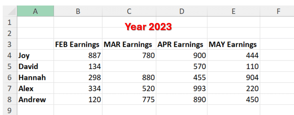
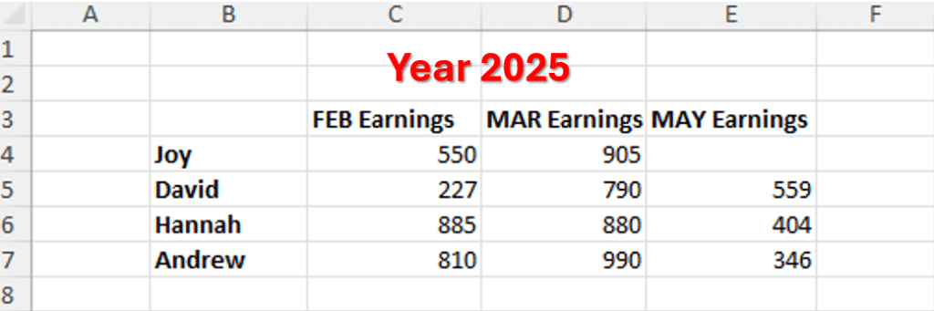
As you can see, we have missing values in C5, D5, and E4 in different worksheets.
This means that David did not receive any commission in March 2023; nor did Hannah in April 2024 or Joy in May 2025. Joy’s row does not appear in Year 2024 and Alex’s is missing in Year 2025. There’s also a missing column in 2025, meaning no employee received commission for April.
Despite all thisExcel can consolidate the information. It can create a summary by following only the labels you’ve created. This feature makes consolidating by category much easier than using formulas.
But before we dive into the nuts and bolts of creating consolidated summaries, there are a few things to note:
- The worksheet tables need to follow a similar layout, where the headings and labels are placed in the same positions.
- You can rearrange the columns and rows, but you need to make sure they have identical names. This means that all labels should have the same spelling and wording.
- Delete any empty rows or columns.
Step 1:
You need to find a separate sheet where the summary table will be located. You can add a new worksheet or rename an existing one.
We’ve named ours ‘‘Summary’’:

Step 2:
Make sure your sheet is empty. Choose the region you want your master sheet to feature. Click on the upper-left, empty cell where your summary table will start to cover.
Step 3:
On the ribbon, go to ‘Data’ then navigate to ‘Consolidate’:
Step 4:
Click the drop-down bar under ‘Function’. You’ll get various choices such as Sum, Min, Count, Max, among others. We’ve selected ‘Sum’ because we need to add the values of all three worksheets together.
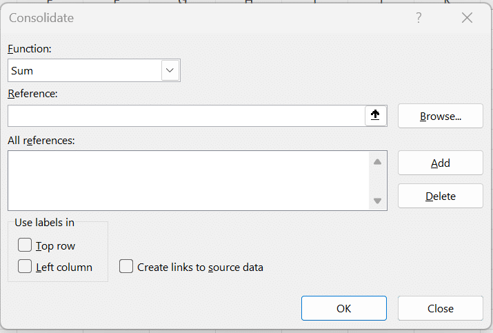
If we wanted the average amount of commissions received by employees over the three years, we’d choose ‘Average’.
Step 5:
Choose a source for Excel to reference. Since our worksheets are on the same file, we navigate to ‘Year 2023,’ our first worksheet.
We’ll then click and drag so that we can highlight the information we’re consolidating. In this case, we’ll select A3 to E8 on the Year 2023 sheet.
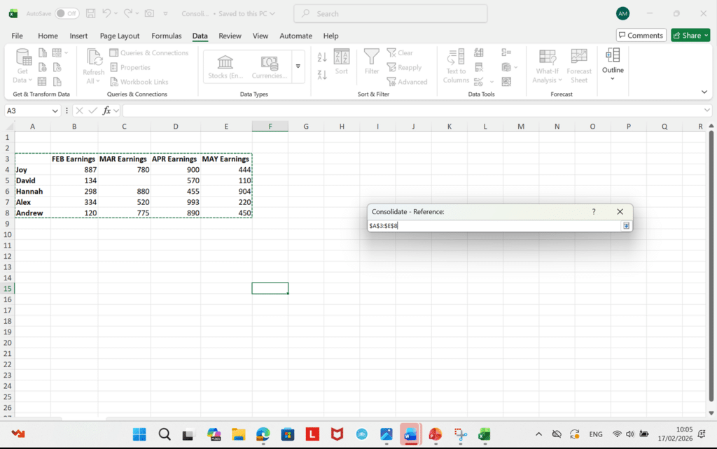
In the reference section, a display will pop up showing your worksheet’s name with an exclamation mark beside it, while also detailing your chosen row and column range. For instance, we get ‘’Year 2023 !$A$3:$E$5”.
If you’re looking to combine data from different files, navigate to ‘Browse’ and select your file. Then click ‘Open’.
Step 6:
Find the ‘Add’ button that’s right next to ‘All References,’then click it. This will include the Year 2023 range in your combined references list.
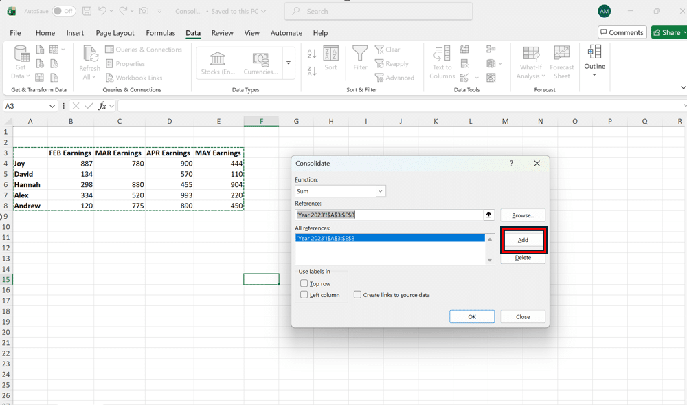
Step 7:
Repeat steps 5, 6, and 7 for the remaining worksheets.
Ensure you add each table as is, without leaving any labels or headings. You’ll get similar recordings in the ‘All References’ section.
Step 8:
Check all the boxes under ‘Use Labels In.’
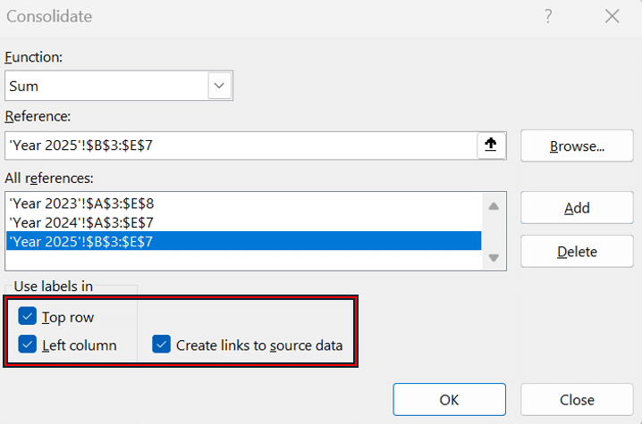
When we check the ‘Top Row’, we enable the consolidation tool to include our labels in the highest rows: February, March, April, and May Earnings.
Likewise, when we check ‘Left Column’, we allow the functionality to include our furthest-left labels: Joy, Hannah, Andrew, Alex, and David.
Selecting the “Create Links’ option enables the platform to update the summary table whenever we change the source information.
If you leave it unchecked, you’ll have to manually update the master worksheet whenever you notice any changes.
Step 9:
Press ‘Ok’ to authorize Excel to consolidate your information in the target worksheet.
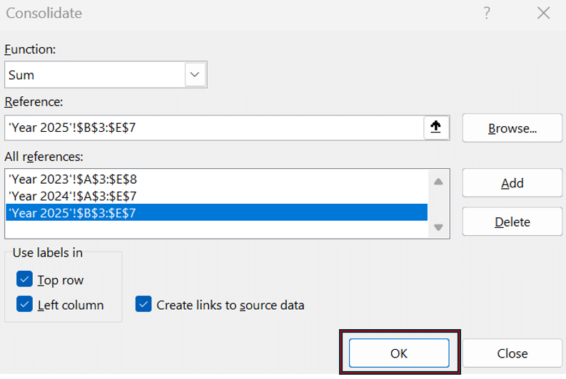
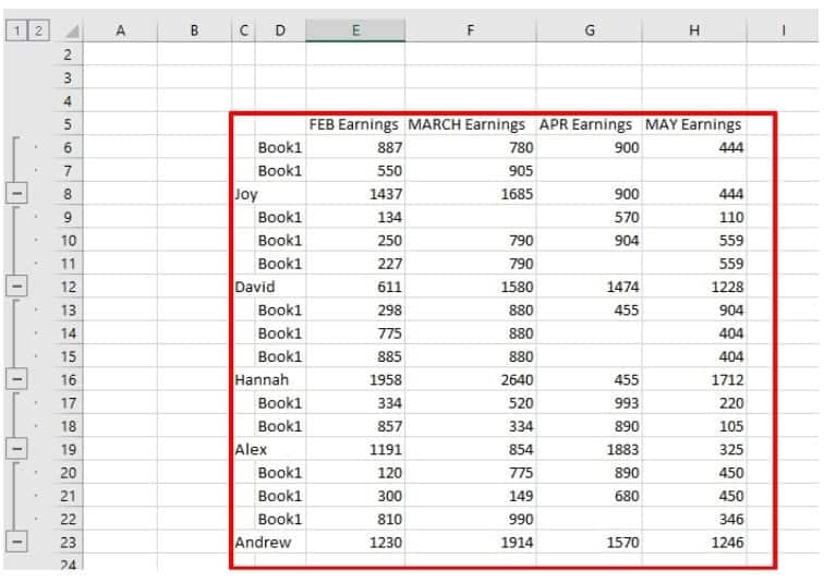
Clicking the ‘+’ buttons next to the cell numbers allows you to view the original information from the new master worksheet.
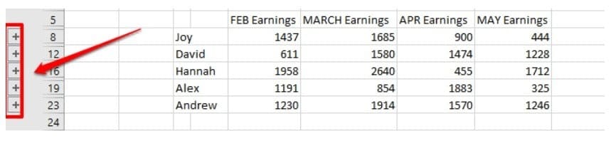
After completing these steps, you’ll get a final product that looks similar to this:
You have to note a few things, though:
- You can create links only when your source information and summary table are in different worksheets. When they’re on the same worksheet, the consolidated information can’t be updated automatically.
- To change the range of your reference, you first have to delete the outline reference in the ‘List’ section before creating one. After deleting it, return it to your sheet and drag it again to get a suitable range.
- If you leave ‘Top Row’ and ‘Left Column’ unchecked, then the platform combines all the cells positioned similarly, such as: cells C5 (Year 2023) + C5 (Year 2024) + C5 (Year 2025). Avoid this by clicking on the boxes.
Excel Consolidation Examples in Finance
To make the concept of data consolidation more concrete, let’s look at a few examples of how finance teams might use Excel to consolidate data:
Monthly Actuals Consolidation
Suppose each department in a company maintains its own Excel sheet for monthly actual expenses.
At the end of the month, the FP&A analyst needs a company-wide actuals report.
Using Excel, the analyst can consolidate these sheets into one master actuals report.
This might be done by linking each department’s total into a summary sheet, or by using the Consolidate function to sum all department figures into one set of totals.
What you get is an aggregated view of actual spending across the whole company for that month.
Multi-Entity Financial Reporting
In a group of companies or a business with subsidiaries, each entity might have its own financial workbook. To prepare consolidated financial statements, finance teams often gather data (such as trial balances and P&L figures) from each entity’s Excel file.
Excel can combine these by summing revenue from all entities to get a group total, while also stacking or categorizing by entity for reporting.
This use case may involve consolidating by category (ensuring that account names or GL codes align so that Excel matches them during consolidation). It works when the chart of accounts is consistent across entities.
Budget vs. Actual Comparison
A classic task in management reporting is comparing budgeted figures to actual results. These often come from different sources (the budget may be in one file, actuals in another).
To consolidate for comparison, you might pull both sets of data into one Excel model.
For example, using formulas or Power Query, combine the budget and actual data, then use a pivot table or summary table to show budget vs. actual variances for each line item.
Here, consolidation might involve aligning data by category, ensuring that each budget line matches the corresponding actual line for a proper comparison.
Rolling Forecast Inputs
In a rolling forecast process, new actuals are added each month, and forecasts are updated for future periods. A finance team might maintain separate forecast files for different business units or scenarios (best-case, worst-case).
To get a consolidated view of the latest forecast, all those pieces need to come together.
In Excel, an analyst might consolidate these by linking each business unit’s forecast into a master forecast workbook.
Alternatively, they might use Power Query to append multiple forecast files into one table, then analyze it. The consolidation ensures that all segments of the business are represented in the single rolling forecast output that management reviews.
In all these examples, Excel can be the glue that combines disparate data into a coherent whole. Each scenario uses a slightly different approach: some use the built-in tool, others use formulas or queries.
However, the principle is that Excel consolidates multiple sources into a single unified report. As long as the underlying data is structured consistently and carefully managed, Excel can handle these consolidation needs for finance teams.
For further reading on improving budgeting and forecasting processes, check out our guide on financial forecasting methods, which can complement effective data consolidation by ensuring your forecast data is organized for easy merging.
Common Challenges When Consolidating Data in Excel
While Excel can certainly get the job done for data consolidation, it’s not without challenges.
Many finance professionals have experienced these pain points when trying to maintain complex consolidated workbooks:
- Manual Updates and Errors: Excel consolidation often involves a lot of manual steps: copying data, entering formulas, adding new links when a new sheet comes in, etc. This manual process is error-prone: a small mistake, such as a mistyped formula or forgetting to update a range, can lead to incorrect results.
- Broken Links and Formulas: As consolidations grow, you might have formulas referencing dozens of external files or far-flung cells. It’s easy for links to break. For example, if someone renames a file or moves it to a different folder, any formulas linking to it will return errors.
- Version Control Issues: When multiple people are contributing data (say, each department submits a spreadsheet), you end up with numerous versions floating around. It can be hard to know which figures are the latest or most accurate.
- Auditability and Transparency: When Excel data rolls up through layers of links and formulas, it’s hard to trace numbers back to their sources. Without built-in audit trails, reviewing or verifying totals becomes time-consuming and unclear, especially under scrutiny.
- Performance Limitations: As data volumes and consolidation complexity increase, Excel can slow down or even crash. Large files with thousands of link formulas and millions of cells of data will tax your computer’s memory. Calculations might take a long time to run, or the file might become unstable.
- Security and Control: Another challenge is ensuring data integrity and security. Excel files can be easily modified (intentionally or accidentally). There’s a risk that someone changes a number in a linked file, and the change is silently reflected in the consolidation.
Why these challenges matter: For finance teams, the cost of a consolidation error can be high; it might mean a misreported financial result or a bad decision due to inaccurate data. The time spent fixing broken Excel links or hunting down the correct version of a file is time not spent on analysis or value-added work.
Being aware of these challenges is the first step; the next is implementing best practices to mitigate them or considering tools that reduce the reliance on fragile processes.
Excel Consolidation Best Practices
If you choose to consolidate data in Excel, following a few best practices can make your life much easier and your results more reliable.
- Use Consistent Data Structures: Standardize layouts across all sheets with matching headers and formats. Consistency reduces errors and simplifies consolidation.
- Avoid Hardcoding Values: Use formulas or links instead of typing numbers. Hardcoded values won’t update and are easy to forget or misinterpret later.
- Use Named Ranges or Tables: Turn data into Excel Tables or define named ranges for clearer, expandable references that adjust as data grows.
- Keep a Separation of Inputs and Summary: Place raw data and summary outputs on separate sheets. This makes tracing, updating, and troubleshooting easier.
- Document Your Process: Add notes or a README tab explaining your sources, methods, and assumptions. It helps with collaboration and review.
- Validate the Results: Double-check totals and match labels to ensure nothing was missed. Reconciliations and spot checks help catch small issues early.
- Limit Complexity Where Possible: Use straightforward formulas and steps. Avoid overbuilding models with excessive links or nested logic.
These best practices help you mitigate some of the common problems of Excel consolidation. The idea is to impose a bit of structure and discipline on Excel’s flexibility, so you still get the benefit of a familiar tool, but with fewer headaches.
Interested in more ways to improve your financial data processes? Read about balance sheet reconciliation to see how consistent data structuring aids in both consolidation and reconciling accounts.
When Excel Stops Scaling for Data Consolidation
As useful as Excel is, there comes a point when relying on spreadsheets alone starts to hold you back. It’s important to recognize when Excel stops scaling for your consolidation needs and when it might be time to consider more robust solutions.
Here are some signs and situations indicating Excel is reaching its limits:
- Too Many Sources to Manage: When consolidating across many departments and files, Excel becomes hard to manage. More sources increase the risk of errors and missed updates.
- Constantly Changing Data: Excel can’t keep up with frequent updates. For daily or weekly consolidations, manual steps are too slow and prone to mistakes.
- Large Data Volumes: Excel can slow down or crash with very large datasets. If it can’t open or process all your data, it’s time to consider a more scalable tool.
- Multiple Entities or Complex Structures: Handling eliminations, currency conversions, and hierarchy roll-ups gets too complex in Excel. Specialized tools manage this better.
- Collaboration and Control Needs: Excel isn’t built for multi-user workflows. Version control, permissions, and approvals are difficult to manage in shared files.
- Audit and Compliance Requirements: Excel lacks built-in audit trails. If tracking changes for compliance becomes a chore, a more structured system is likely needed.
In these situations, continuing to push Excel further can lead to significant risks. You may encounter situations like data being out-of-sync because someone forgot to send an updated file, or a consolidation that takes so long to run that you miss reporting deadlines.
Excel stops being efficient and starts being a liability.
How Modern Finance Teams Consolidate Data Today
While Excel isn’t going anywhere, many SMEs opt to enhance it with more advanced data consolidation solutions.
Here’s how forward-thinking teams are handling consolidation:
- Automation with ETL and Integration Tools: ETL tools pull and transform data from multiple systems into a central database, eliminating manual steps and keeping data consistent and current.
- FP&A and CPM Systems: Tools like Datarails automate consolidation by pulling data from many sources and pushing results into Excel templates or dashboards, saving time and improving accuracy.
- Power Query and Power BI: Power Query and Power BI help teams consolidate, shape, and visualize data from multiple files or systems, with automation and reporting built into the process.
- Cloud Collaboration: Shared tools like Google Sheets or Excel Online reduce version issues and let teams work from one live file, though advanced Excel features may be limited.
- Controlled Data Models: Central data models store cleaned and structured data that Excel can pull from, shifting consolidation away from spreadsheets and into scalable databases.
- Maintaining Excel for Front-End Flexibility: Many teams still use Excel for reporting, but now rely on tools like Datarails to automate the data feeding process, blending flexibility with consistency.
Modern consolidation is about automation, accuracy, and timeliness. Finance teams realize that spending two weeks gathering and verifying numbers is not a good use of time or talent, especially when closing the books or reforecasting quickly is critical.
By investing in tools and processes that streamline consolidation, they can reallocate time to analyzing results and advising the business.
These software solutions also add features like audit trails, user permissions, and scenario management, which Excel struggles with, thereby strengthening control over the financial data.
Working manually on most spreadsheet tasks can be overwhelming, tiring, and repetitive.
Datarails automates time-consuming Excel work, enabling you to deliver error-free work and focus on more strategic tasks. The best part? You don’t have to change your processes and keep on using Excel.
Streamline the connection between your company’s finance and operations and encourage better organization decisions with Datarails FP&A Software.
Excel Data Consolidation FAQs
Use the Consolidate tool under the Data tab to combine ranges from multiple sheets or workbooks using functions like SUM or AVERAGE. Make sure your data has a consistent layout, then select your ranges and let Excel create a summary.
You can also use formulas, PivotTables, or Power Query, depending on your setup.
It depends on your data:
– The Consolidate feature is great for consistent layouts
– Formulas offer flexibility
– PivotTables help with grouping
– Power Query is best for automation
Many teams use a mix of these tools based on the task.
Yes, Excel can consolidate across workbooks using the Consolidate tool or formulas. You can link to other files or use Power Query to pull from folders if you’re working with many files. Just be sure your external files are accessible and saved.
Power Query helps you pull, clean, and combine data from multiple sources into a single table. It’s especially useful for repeated consolidations, since you can refresh queries without having to redo steps.
It’s a powerful automation tool built into Excel.
Manual consolidation is slow and prone to errors, like broken formulas or outdated files. It also lacks transparency, making audits difficult and version control a challenge. These risks grow with scale, which is why automation is often preferred.
Excel works well for small or mid-sized tasks with a clear structure. It offers flexibility through formulas and PivotTables, and many teams rely on it for early-stage or ad-hoc consolidation. But it struggles with scale, complexity, and frequent updates.
Move on when Excel becomes slow, error-prone, or hard to manage due to frequent updates, growing data, or team collaboration. If you’re spending more time fixing errors than analyzing data, it’s time to upgrade.
Datarails can automate consolidation while still letting you use Excel for reporting.